ClockBoard: a zoning system for urban analysis

Robin Lovelace

Institute for Transport Studies and Leeds Institute for Data Analytics, University of Leeds, UK

Martijn Tennekes

Center for Big Data Statistics, Centraal Bureau voor de Statistiek, The Netherlands

Dustin Carlino

Independent Software Engineer, Lead Developer of A/B Street, USA

Abstract

Zones are the building blocks of urban analysis. Fields ranging from demographics to transport planning routinely use zones — spatially contiguous areal units that break-up continuous space into discrete chunks — as the foundation for diverse analysis techniques. Key methods such as origin-destination analysis and choropleth mapping rely on zones with appropriate sizes, shapes and coverage. However, existing zoning systems are sub-optimal in many urban analysis contexts, for three main reasons: 1) administrative zoning systems are often based on somewhat arbitrary factors; 2) zoning systems that are evidence-based (e.g. based on equal population size) are often highly variable in size and shape, reducing their utility for inter-city comparison; and 3) official zoning systems in many places simply do not exist or are unavailable. We set out to develop a fexible, open and scalable solution to these problems. The result is the ClockBoard zoning system, which consists of 12 segments emanating from a central place and divided by concentric rings with radii that increase in line with the triangular number sequence (1, 3, 6 km etc). ‘ClockBoards’ thus create a consistent visual frame of reference for monocentric cities that is reminiscent of clocks and a dartboard. This paper outlines the design and potential uses of the ClockBoard zoning system in the historical context, and discusses future avenues for research into the design and assessment of zoning systems.

Introduction

Zoning systems have long been used for a variety of administrative and practical purposes. Zones demarcating parcels of land have been integral to land ownership, rents and urban policies for centuries, forming the basis of a range of social and economic practices. Historical examples highlighting the importance of zone layouts include ‘tithe maps’ determining land ownership and taxes in 18th Century England (Bryant and Noke 2007) and the division of cities into discrete areas including legally defined “business, industrial, and residential zones” to tame chaotic urban growth in the exploding US cities in the early 1900s (Baker 1925).

In the 19th Century, zoning systems became known for political reasons, with ‘gerrymandering’ entering public discourse and academic research following Elbridge Gerry’s apparent attempt to gain political advantage by creating an electoral district in an odd shape that was said to resemble a salamander (hence the term’s name combining ‘Gerry’ and ‘salamander’) in 1812 (Orr 1969). Gerrymandering has since been the topic of countless academic papers that is the beyond the scope of the present paper.

Research has made great progress in mathematical analysis of zones and more objective assessment of the impacts that the nature of zoning systems can have on zone-based statistics (such as number of votes for a particular party in each zone) and outcomes. The gerrymandering problem (in itself is a manifestation of the modifiable area unit problem) can be described as a mathematical optimization problem: “\(n\) units are grouped into \(k\) zones such that some cost function is optimized, subject to constraints on the topology of the zones” (Chou and Li 2006). Prior work has demonstrated the sensitivity of urban analysis outcomes to zone system design, from the way cities are visualized to the impact of the nature of ‘traffic analysis zones’ on transport model outputs. In fact, this problem is a concise definition of the broader “zoning problem” that starts from the assumption that zones are to be composed of one or more basic statistical units (BSUs) (Jelinski and Wu 1996; Chandra et al. 2021) . Although the range of outcomes is a finite combinatorial optimisation problem (which combination of BSU-zone aggregations satisfy/optimize some pre-determined criteria) the zoning problem is still hard: “there are a tremendously large number of alternative partitions, a similar number of different results, and only a slightly smaller number of different interpretations” (Openshaw 1977).

The problem that we tackle in this paper is different, however. It is ‘zoning from scratch’: the division of geographic space into zones starting from a blank slate, without reference to pre-existing areal units. The focus of much preceding zoning research on BSU partitioning can be explained by the fact that much geographic data available to academics comes in ‘pre-packaged’ small areas and because creating zones from nothing is a harder problem. We disagree with the statement that “existence of individual or non-spatially aggregated data is rare in geography” (Openshaw 1977), pointing to car crashes, shop locations, species identification data and dozens of other phenomena that can be understood as ‘point pattern processes’. And with advances in computer hardware and software, the ‘starting from scratch’ approach to zoning systems is more feasible.

A number of approaches have tackled the question of how to best divide up geographical space for analysis and visualisation purposes, with a variety of applications. Functional zone classification is common in the field of remote sensing and associated sub-fields involved in analysing and classifying raster datasets (Ciglic et al. 2019; Hesselbarth et al. 2019). While such pixel-based approaches can yield complex and flexible results (depending on the geographic resolution of the input data), they are still constrained by the building blocks of the pixels, which can be seen as a particular type of areal unit, a uniformly sized and shaped BSU.

In this paper we are interested in the division of continuous space into completely new areal systems. This has been done using contour lines to represent lines of equal height, and the concept’s generalisation to lines of equal journey time from locations (isochrones) (Long 2018), population density (isopleths) (Lin, Hanink, and Cromley 2017) and model parameters which continuous geographical space (P’aez 2006). The boundaries created by these various ‘iso’ maps are ‘procedurally generated’ areal units of the type that this paper focuses, but their variability and often irregular shapes make them impractical for many types of urban analysis.

Procedural generation, which involves the generation of data through a repeated and sometimes randomized computational process has long been used to represent physical phenomena (Onrust et al. 2017). The approach has been used to generate spatial entities including roads (Galin et al. 2010), indoor layouts of buildings (Anderson et al. 2018) and urban layouts (Mustafa et al. 2020). Algorithms have also been developed to place linear features on a map, as illustrated by an algorithm that optimizes the placement of overlapping linear features for cartographic visualisation (Teulade-Denantes, Maudet, and Duchêne 2015). However, no previous research has demonstrated the creation of zoning systems specifically for the purposes of urban analysis.

New visualisation techniques are needed to represent new (or newly quantifiable) concepts and emerging datasets (such as OpenStreetMap) in urban analysis. The visualisation of direction has been driven by new navigational requirements and datasets, with circular compasses and displays common in land and sea navigational systems since the mid 1900s (Honick 1967). Circular visualisation techniques, in the form of rose diagrams, were used in a more recent study to indicate the most common road directions relative to North (Boeing 2021). The resulting visualisations are attractive and easy to interpret, but are not geographical, in the sense that they cannot meaningfully be overlaid on mapped data. The approach we present in this paper is more closely analogous to ‘grid sample’ approaches used in ecological and population research (Hirzel and Guisan 2002) . Historically, environmental researchers have used rectangular (and usually square) grids to divide up space and decide sampling strategies. Limitations associated with this simplistic strategy have been documented since at least the 1960s, with a prominent paper on geographic sampling strategies outlining advantages and disadvantages of simple random, systematic and stratified sampling techniques in 1967 (Holmes 1967). Starting with data at the level of raster grid cells and BSUs, a related approach is to sample from within available ‘pixels’ to generate a representative sample (Thomson et al. 2017).

Unlike BSU based zoning systems, grid sampling strategies require no prior zones. Unlike ‘procedurally generated’ areas, grid-based strategies generate areal units of consistent sizes and shapes. However, grid-based strategies are limited in their applicability to urban research because they seldom generate geographically contiguous results and do not account for the strong tendency of human settlements to have a (more-or-less clearly demarcated) central location with higher levels of activity.

Pre-existing zoning systems are often based on administrative regions. Although those zoning systems are usually in line with the hierarchical organization structure of governmental organizations, and therefore may work well for policy making, there are a couple of downsides to using such zoning systems. First of all, since a city and its politics change over time, the administrative regions often change accordingly. This makes it harder to do time series analysis. Since the administrative regions have heterogeneous characteristics, for instance population size, area size, proximity to the city centre, comparing different administrative regions within a city is not straightforward. Moreover, comparing administrative regions across cities is even more challenging: the average surface area of a administrative zones varies from city to city.

Grid tiles are popular in spatial statistics for a number of reasons. Most importantly the tiles have a constant area size, which makes comparably possible. Moreover, the grid tiles will not change over time like administrative regions. However, one downside is that a grid requires a coordinate reference system (CRS), enforcing (approximately) equal area size. For continents or large countries, a CRS is always a compromise. Therefore, the areas of the tiles may vary, or the shape of the tiles may be sheared or warped.

Another downside from a statistical point of view is that population densities are not uniform within a urban area, but concentrated around a centre. As a consequence, high resolution statistics is preferable in the dense areas, i.e. the centre, and lower resolution statistics in other parts of the city. That is the reason why administrative regions are often smaller in dense areas.

The approach presented in this paper aims to miniminput data requirements, generate consistent zones comparable between widely varying urban systems, and provide geographically contiguous areal units. The motivations for generating a new zoning system and use cases envisioned include:

• Locating cities. Automated zoning systems based on a clear centrepoint can support map interpretation by making it immediately clear where the city centre is, and what the scale of the city is.

• Reference system for everyday life. The zone name contains information about the distance to the center as well as the cardinal direction. E.g “I live in C12 and work in B3.” or “The train station is in the center and our hotel is in B7”. Moreover, the zones indicate whether walking and cycling is a feasible option regarding the distance.

• Aggregation for descriptive statistics / comparability over cities. By using the zoning system to aggregate statistics (e.g. on population density, air quality, bicycle use, number of dwellings), cities can easily be compared to each other.

• Modelling urban cities. The zoning system can be used to model urban mobility.

The paper is structured as follows. The next section outlines the approach, which requires only 2 inputs: the coordinates of the central place in the urban system under investigation, and the minimum radius from that central point that the zoning system should extend. Section 3 describes a number of potential applications, ranging from rudimentary navigation and location identification to mobility analysis. Finally, in Section 4, we discuss limitations of the approach and possible directions of research and development to generate additional zoning systems for urban analysis.

The ClockBoard zoning system

The aim of the ClockBoard zoning system is to tackle the issues associated with available zoning systems and to provide a standard template for research and communication purposes. The requirements of urban analysts, geographers, transport modellers and others working with geographic data across cities are diverse, but all rely on zoning systems as a foundation for modelling and visualisation. To enable flexibility, and to encourage other zoning systems building on it, the ClockBoard zoning system described in this paper is presented as a specific implementation of a more general concept (segmented concentric annuli) and implemented in open source software which can be extended in a range of ways (see Discussion). Considering urban analysis, modelling and wider research, visualisation and communication requirements of zoning systems, we developed the following criteria for successful zoning systems. Zoning systems for urban analysis should:

• contain intuitively named zones, enabling public communication of research, e.g. with reference common perceptions of space in terms of distance from the city centre and direction relative to North
• have a well-balanced number of zones since too many or too few zones may cause issues with analysis and visualisation be easy to visualize without too many or too few zones
• include zones of consistent and useful sizes, for example with zone areas increasing with distance from the urban centres to reflect relatively high densities in central locations
• be ‘scale agnostic’, capable of representing a range of urban forms ranging from extensive cities such as Mexico City to compact cities such as Hong Kong
• be extensible and based on open source software, enabling others to create alternative zoning systems suited to diverse needs

Considering the above criteria, we explored many zoning options, some of which are illustrated in Figure 1. Two key concepts that make up the zoning system described in this paper are concentric annuli and segments defined by radii.

• Concentric rings — formally called ‘concentric annuli’ — which emphasise central locations and have been used to explore the relationships between the characteristics of ‘focal trees’ and surrounding trees in ecological research (Wills et al. 2016), as shown in Figure 1 (A).

• Segments, defined by radial lines emanating from the central point of the settlement (or other geographic entity) to be divided into zones, as shown in Figure 1 (B).

Combining these two concepts creates a general approach to zone creation that can be described as ‘segmented concentric annuli’, an implementation of which that we considered early in the process of designing the ClockBoard system with roughly equally sized zones (not the ClockBoard system) is shown in Figure 1 (C). After a period of informal testing and feedback that lasted approximately six months, we developed and refined the ‘ClockBoard’ zoning system presented in this paper, which is a specific implementation of the segmented concentric annuli approach to zone creation.

The parameters that define the ClockBoard zoning system were developed in an iterative process. We experimented with a range of ways of dividing the concentric annuli into different zones by modifying the distances between rings (the annuli borders) and the number of segments per annulus. It became apparent that zoning systems based on the two organising principles (and modifiable parameters) of concentric annuli and segments held promise, but selecting appropriate settings for each was key to the development of the ClockBoad zoning system, as outlined below.

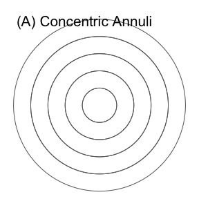
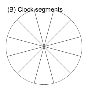
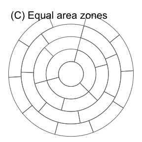
Figure 1: Illustration of ideas explored in the lead-up to the development of the ClockBoard zoning system, highlighting the incremental and iterative evolution of the approach.

Annuli radii

Each annuli is defined by its inner and outer circle. Given that the radius of the inner circle must the same as the radius of the preceding annuli to ensure geographically contiguity (no gaps) — except in the special case of the first and central annuli which has no inner circle (or an inner circle with a radius of zero) — the annuli sizes can be wholly defined by the sequence of numbers defining their out circle radii.

This sequence of numbers can increase by a fixed amount — e.g. with the outer border of each annuli being 1 km from the centre than the preceding annulus, as shown in Figure 1 (C) — or by varying amounts. In many cases it is useful for zones to be smaller near the centre of the study region surrounding cities. This truism is often reflected in traffic analysis zones (TAZ) used for transport modelling, which tend to be smaller near central areas where more detail is most important for policy-relevant outputs (Chandra et al. 2021).

After experimenting with various ways of incrementing the annuli width, and considering the importance of easy to remember distances from central points from the perspective of readability, interpretation and simplicity of the system, we settled on linear increases in width as a sensible default for the ClockBoard zoning system. This linear growth leads to distances between the outer circles of each annuli and the central point following in the triangular number sequence (Ross and Knott 2019). This means that all points in the first annuli (labelled A) are up to 1 km away from the city centre; a circle with a diameter of 1 km is an easy to remember (albeit not always accurate) way to define the central area of urban areas (Vinoth Kumar, Pathan, and Bhanderi 2007). The furthest points from the central point of the next 8 subsequent annuli in the system (annuli B to I) are 3, 6, 10, 15, 21, 28, 36 and 45 km respectively, meaning that even a large city such as London requires only 8 annuli to cover it entirely (Figure 2). This and other other attributes of the first set of 9 zones in the ClockBoard zoning system in Table 1.

Table 1: Key attributes of first 9 rings used in the ClockBoard zoning system.

N. annuli	Outer annuli label	N. zones	Radius (km)	Area (sqkm)	Average zone size (km)
1	A	1	1	3	3
2	B	13	3	28	2
3	C	25	6	113	5
4	D	37	10	314	8
5	E	49	15	707	14
6	F	61	21	1385	23
7	G	73	28	2463	34
8	H	85	36	4072	48
9	I	97	45	6362	66

Number of segments

As its name suggests, the ClockBoard zoning system has 12 segments, representing a compromise between specificity of zone identification and ease of comprehension. On one hand, too few segments result in large and/or unusually shaped zones, as illustrated in a segmented concentric annuli zoning system with four segments per annuli developed by Vinoth Kumar, Pathan, and Bhanderi (2007) to model urban expansion. On the other hand, too many segments would result in small zones and make the zone codes harder to understand: imagine a system with 256 segments and saying “I’m in zone E173”!

Another advantage of using 12 segments is that the angular distance between segments are well understood. The ‘clock position’ system describes bearings with reference to the face of a clock, relative to the direction of travel or, as is the case with the ClockBoard zoning system, relative to true North. Under this system, well established in navigation, “12 O’clock” means true North and 3, 6 and 9 O’clock mean East, South and West respectively (Hart and Battiste 1991). Following this convention, the ClockBoard zoning system aligns segment 12 with true North, enabling users to approximate their location in a city with reference to clock position .

ClockBoard zones for segmenting urban areas

The result of applying 12 segments and n concentric rings with external diameter increasing as triangular numbers, with n being sufficient to cover the city extent with, is the Clockboard zoning system. As outlined in the Introduction, the primary motivation for developing the system was urban analysis and the description, visualisation and exploratory analysis of large cities with well-defined central areas such as London, as illustrated in Figure 2.

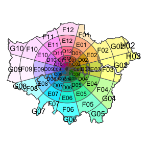
Figure 2: The clockboard zoning system, applied to Greater London, UK.

Using the ClockBoard zoning system

To enable easy access to the ClockBoard zoning system, we implemented techniques needed to create them in free and open source software. The tools described below allow people to create ClockBoards in a reproducible way from command line environments and even from a web browser, to minimise barriers to entry.

The zonebuilder R package

The concepts were initially implemented in the statistical programming language R, which is available from the Comprehensive R Archive Network (CRAN) and can be installed from the R command line as follows:

install.packages("zonebuilder")

After the package has been installed, its functions can be attached (made available) to the user’s workspace as follows:

library(zonebuilder)

A simple zoning system for Tokyo can be created as follows, resulting in the map shown in Figure 3:

ClockBoard_tokyo = zb_zone("Tokyo", n_circles = 5)

Figure 3: ClockBoard zoning system applied to Tokyo, the result of running the reproducible code used to demonstrate the zonebuilder R package.

Note that the n_circles argument was set to 5, resulting in a zoning system 15 km in radius (see Table 1). This can be changed; replacing 5 with 9, for example, would results in a zoning system with an outer circle radius of 45 km. Furthermore, passing an object representing the geographic extent of Tokyo as a polygon to the area argument of the zb_zone() function would result in a zoning system that is intersected by Tokyo’s boundary.

The zonebuilder Rust crate

To make the project and resulting zones available to more people, we subsequently developed a Rust crate, that enables the creation of ClockBoard zones on all major platforms using a command line interface. See github.com/zonebuilders/zonebuilder-rust for details. The crate is available on the main Rust package repository crates.io and can be installed on any computer that already has the Rust toolchain installed from the system command line as follows:

cargo install zonebuilder

After installing the zonebuilder crate and assuming that cargo is executable the following commands will print instructions on how to use the command line interface and generate zones for Leeds, UK, respectively:

zonebuilder -h               # see usage instructions
zonebuilder > zones.geojson  # create zones.geojson zone object

Interactive zonebuilder web application

To enable creation of ClockBoard zones for non-programmers and to encourage people to explore alternative zoning systems, we created a simple web application hosted at zonebuilders.github.io/zonebuilder-rust/ (see Figure 4). This app leverages the Rust implementation for generating ClockBoards, compiling it to WebAssembly and using the standard open-source leafletjs.com mapping library as an interface.

Figure 4: Screenshot of the zonebuilder web application for creating and downloading ClockBoard zones interactively. The example shows Erbil, Northern Iraq, which was found to have a road layout resembling the ClockBoard zoning system, highlighting the importance of interactive alignment and selection of number of rints. See the interactive version at zonebuilders.github.io/zonebuilder-rust/.

Applications

The zoning system presented in this paper is a specific implementation concentric segmented annuli, that was designed to support description, exploration and visualisation of monocentric cities. The zoning system presented, and modifications of the system, could be useful in a range of other areas. The examples below are designed to provide an insight into how the zoning system could be used.

Navigation and location

The most basic application of the zoning system could be to provide approximate locations and navigation guidance to people in cities. As demonstrated by location services such as ‘what3words’ and open source implementations such as ‘whatfreewords’ and ‘goehashphrase’, there is demand for easy-to-remember words/phrases to specify locations in situations where there is no address and where providing longitude/latitude coordinates may not be appropriate or possible (Raposo, C. Robinson, and Brown 2019). While not the primary purpose of the ClockBoard zoning system, it can be used to communicate locations in a city.

We have tested this use case by using the zoning system to agree on meeting points to collaborate on the project. An illustration of how the zoning system was used is shown in Figure 5, which shows how the ClockBoard zoning system could be used to communicate key locations in a city, from the train station (zone A) to a park (zone C01) and on to the city of Bradford (zone E09) to orientate people new to the city and to describe geographically where things are located using a small amount of information (3 characters). Without needing to process much data or look at the map, a person who is new to to the city would know that the park is relatively close to the rail station (between 3 and 6 km from the city centre) while Bradford in zone E09 is between 15 and 21 km from the city centre. Note that although Bradford is a city on its own and can therefore have its own zoning system, in this example it is placed in the context of the metropolitan area of Leeds. Of course the locations are not geographically specific; the zones would be used a broad brush descriptions of place locations before more detailed locations are provided, e.g. through a postcode, an address, or coordinates.

Figure 5: Illustration of how the ClockBoard system could be used to describe the approximate location of places. In this hypothetical example, someone is describing key places to visit in and around Leeds to someone who arrives at the train station in zone A, visits the city’s famous Roundhay Park in zone C01, before travelling for an evening meal in Bradford, in zone E09.

Exploring city scale data

The ClockBoard zoning system is well suited to exploratory analysis of city-scale spatial data. An example that demonstrates how the system can simplify the presentation of spatially variable data is shown in Figure 6, which presents open access data on air quality from the London Atmospheric Emissions Inventory. The presentation of the same data at four different levels of geographic resolution highlights the impacts that zoning system choice can have on data analysis, with each having advantages and disadvantages. The most geographically detailed zoning system in which the data is available is the rectangular grid shown in the far left facet (A). This presentation of the data is ideal for many purposes, demonstrating the variability in air quality over relatively small areas (1 km grid cells) across London.

In cases when geographic aggregation is required, e.g. to present the data in small graphics that will be printed at low resolution (e.g. newspaper visualisations and infographics), two common approaches are to use an existing administrative zoning system (with well known London Borough boundaries used to aggregate the data presented in facet B in Figure 6) and to use a simplified geographical representation or geographically arranged facets (Dorling 2011). Both approaches have advantages, with existing and well-known zoning systems enabling map readers familiar with the city to orient themselves and interpret the map. In this context and with reference to Figure 6, the ClockBoard zoning system has the following advantages as a basis for choropleth maps:

• Simple and consistent zone shapes for easy map reading
• The circular shape of zone boundaries make the results easy to place, requiring a 1:1 aspect ratio (except when the zones are clipped, as in map D)
• The shape of the zones draws attention to citywide spatial patterns, with map C highlighting the clear tendency for air quality to improve with distance from the city centre and the comparatively poor air quality in segments 3 and 9

The final advantage is particularly notable when comparing the ClockBoard zoning system with large official zone (borough) boundaries in London. Because of the large and irregular zone shapes in map B, the strength of the relationship between distance from central London and air quality is not as clear as when using ClockBoard zones as the frame of reference in maps C and D in Figure 6. This benefit is especially noticeable towards the outskirts of London, where large outer boroughs such as Bromley (far southeast London) fail to communicate the fact that PM10 levels drop below 1 ug/m^3 in outer London.

Figure 6: Illustration of the ClockBoard zoning system used to visualize a geographically dependendent phenomena: air quality, measured in mass of PM10 particles, measured in micrograms per cubic meter, from the London Atmospheric Emissions Inventory (LAEI). The facets show the data in spatial grid available from the LAEI, facet Am and aggregated to London boroughs B, to ClockBoard zones covering all the input data shown in C, and ClockBoard zones clipped by the administrative boundary of Greater London in D.

The example of air quality presented in Figure 6 highlights that the ClockBoard zoning system is well suited for the analysis and visualisation of phenomena in which a central place (London city centre in this case) plays a major role, directly or indirectly. (Not all cities have a ‘monocentric’ structure, something we discuss in Section ??.) The prevalence of particulate matter in the air relates to the level of industrial, transport and other activities in the surrounding area, which clearly increases with proximity to central London. The same can be said of many other phenomena which become more, less, or more and then less, common with distance from central places. The tragic phenomena of road traffic casualties — which relate to travel volumes, speeds and transport infrastructure design — also relates (albeit in different ways in different cities) to proximity to central places, something we explore in the next subsection to highlight another use of the ClockBoard zoning system: comparison between cities.

Inter-city comparison of geographically variable phenomena

The ClockBoard zoning system can enable effective comparison between cities by providing a consistent frame of reference. While official boundaries can vary greatly in size and shape, based on sometimes arbitrary factors such as historic boundaries, ClockBoard zones are always the same size, shape and orientation. Using the system can provide a basis of evidence-based discussion of a wide range of phenomena. The example shown in Figure 7 demonstrates this with reference to a policy-relevant example: the number of people killed and seriously injured while cycling in major UK cities. Addressing issues associated with reporting only number of casualties per unit area, a practice that can miss dangerous places which have a high casualty rate per unit time or distance cycled (Mindell, Leslie, and Wardlaw 2012), we show data on the number of people killed and seriously injured while cycling per billion kilometres based on estimates from the Propensity to Cycle Tool (Lovelace et al. 2017).

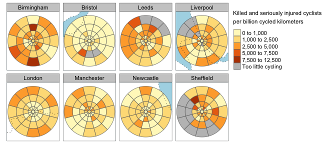
Figure 7: Use of the ClockBoard zoning system to support inter-city comparison of policy-relevant data, on road traffic casualties. The maps show the spatial distribution of cycling casualties per billion km cycled, a measure that requires spatial data aggregation for meaningful results.

The results illustrated in Figure 7 show that while London has a high absolute crash rate, it is relatively safe per km cycled. The ClockBoard zoning system also allows for aggregation at a consistent spatial resolution, enabling the identification of potential crash hotspots in specific parts of Birmingham (zones D12 and E06) and Sheffield (zone D11).

Another example of using ClockBoards to compare cities (and phenomena that take place in them) is shown in Figure 8, which shows population density in 36 major cities using the ClockBoard zoning system not as unit for aggregation but as a reference grid. The 7 rings A to G cover a radius up to 28 km from the city centre. The colors of the panel labels in Figure 8 indicate the continent of the city. The value of comparing cities in a single geographic frame of reference is shown by inspecting Singapore and Sydney with reference to ClockBoard zones. While these cities have similar total official populations (of 5.8 and 5.3 million people, respectively), based on the number of people with their respective administrative boundaries, the size and shape of each city is very different, highlighted by the fact that in Singapore there are few people beyond ring F (located 15 to 20 km from the centre), while in Sydney (and many other cities) there are substantial numbers of people living in ring I (located 36 to 45 km from the centre).

Figure 8: ClockBoard for 36 cities. The blue raster grid cells represent open access population estimates from the WorldPop project.

The administrative borders of six cities shown in Figure 8 are depicted as red lines in Figure 9, highlighting the importance of sometimes arbitrary city boundaries. The ClockBoard zones applied to Amsterdam not only cover Amsterdam but also a few other small Dutch cities and towns. Most of them are economically attached to Amsterdam, but a few of them also to other major Dutch cites.

The benefits of using a single zoning systems across multiple cities is highlighted by comparing London and Paris. Official figures suggest that the two cities have very different sizes: the population within their official boundaries depicted in Figure 9 are 9 million (Greater London) and 2 million (Paris). However, the metropolitan population, which we define as the population living in the ClockBoard zones (within 28 km from the city centre) of those two cities are similar (about 10 million each). The example highlights the utility of ClockBoard for communicating not only inter-city differences in the magnitude and spatial distribution of phenomena, but also geographical extent.

Figure 9: ClockBoard for 6 cities with boundaries shown in red. The blue raster grid cells represent open access population estimates from the WorldPop project; the red lines are administrative borders.

Discussion and conclusion

The ClockBoard zoning system presented in this paper was designed to overcome some well known and long standing issues associated with commonly available administrative zoning systems (Openshaw 1977; Jelinski and Wu 1996). Despite over 100 years of use in some places, and their design not responding to growth in changes in cities in many others, administrative zoning systems are still often used as the default unit of analysis for urban analysis in many parts of the world. Instead of tackling the problem by developing new ways to aggregate basic statistical units (BSUs, the basic building blocks of hierarchical administrative zoning systems) the approach taken in this paper is to start from a blank slate and design zoning systems from scratch, with the aim of creating zones that would be intuitively labelled, of consistent size and shape for creating readable and easy-to-interpret maps, and focussed on the central point on monocentric cities.

Based on these criteria the ClockBoard zoning systems was developed, which consists of regularly spaced rings forming ‘dohnuts’ (technically annuli) emanating from the city centre and labelled A, B, C etc. At the centre of the ClockBoard zoning system lies zone A, a circle measuring 1 km in radius. Beyond zone A, each circular annuli is devided 12 evenly spaced segments labelled 1 to 12, with segment 12 representing land due North of the zone A. The ClockBoard zoning system is a specific implementation of an approach to zone creation that we label concentric segmented annuli; adjusting the sequence of outer ring diameters and number of segments could result in a wide range of alternative zoning systems, each of which would have advantages and disadvantages, just as the ClockBoard zoning system does.

Any such circular zoning system can provide a consistent geographic frame of reference for monocentric cities, or indeed any geographic system with a clear central point. The zones in the ClockBoard zoning system were designed to be sufficiently large so that each could be seen when printed in a low resolution map representing a large city. The relatively large zones (which get bigger further from the city centre as density of urban phenomena tends to decrease) also enables labels that are easy to communicate. Zone labels contain only three characters (with the exception of zone A) and and clearly demarcate the location of phenomena in terms of angle and distance from the centre, with zone C09 located between 3 and 6 km to the West of the city centre. The even growth of rings also enable understanding of the scale of cities and urban phenomena within them, regardless of the size of often arbitrary and historic official boundaries; the first nine rings in the zoning systems (labelled A, B, … I) grow at constant rate, with radii of 1, 3, 6, 10, 15, 21, 28, 36 and 45 km. The consistency of zone sizes and shapes, and the uniform sizes of all ClockBoards that share the same number of rings, could enable more objective and easier to interpret inter-city comparison projects.

The ClockBoard zoning system is not without limitations, however: it represents a series of compromises in which the tendency was towards simplicity and ease of understanding. Perhaps the biggest limitation of the system is its implicit assumption that cities are monocentric entities in which urban activity (and hence the need for spatial resolution) declines gradually with distance from the city centre. While this assumption broadly holds for phenomena such as air pollution in London, as illustrated in Figure 6, it needs to be relaxed in many other cases (Alidadi and Dadashpoor 2018). The ClockBoard zoning system can thus be seen as a zoning system best suited for the analysis of monocentric cities, rather than polycentric conurbations.

A question for further research is how to fit one or several ClockBoards to a dense urban area consisting of several cities, of which none is clearly dominant. For instance, the four major cities in the Netherlands (Amsterdam, Rotterdam, The Hague and Utrecht) are small and located about 40 kilometers from each other, with even smaller cities and towns in between. In this example, there is no dominant “gravitational force” to construct one ClockBoard around. ClockBoards could be constructed for each of these four cities, raising the question: how to design zoning systems for polycentric regions, or large regions that contain multiple monocentric settlements (Chandra et al. 2021)? We explored the possibility of ‘joining’ ClockBoard systems that met, with the ‘dominant’ ClockBoard associated with the larger city, but the results were not promising and we suspect that a new approach altogether, perhaps building on experience from Computational Fluid Dynamics, where grid generation procedures need to take into account multiltiple factors (Hernandez-Perez, Abdulkadir, and Azzopardi 2011).

An alternative and approach to developing zoning systems for complex and polycentric settlements not implemented in this paper is to build them on exisiting Discrete Global Grid Systems (DGGS) such as the S2 and H3 global zoning systems developed by Google and Uber respectively (Bondaruk, Roberts, and Robertson 2020), and the QTM Generator developed by Paulo Raposo (Raposo, C. Robinson, and Brown 2019). This would have advantages for flexibility, with DGGSs able to generate grids with zone sizes that are more evidence-based, for example by respondingM to geographic data such as population density. DGGS based zoning systems would also enable greater determinism, with each of S2’s ~7 quintillion (\(6 * 4^{30}\) or \(\approx6.9*10^{18}\)) and H3’s ~700 trillion (\(\approx5.7 * 10^{14}\)) base zones having a unique reference code that is machine readable (ClockBoards are arguably deterministic with ‘zone B12, Leeds, UK’ referring to an unambiguous area, although ClockBoards depend on an unambiguous definition of ‘city centre’ which may not be available or requires a single unique source of city centre points). Theses beneficial features would be gained at the expense of simplicity: DGGSs are complex and have hard-to-remember cell IDs such as e66ef376f790adf8a5af7fca9e6e422c03c9143f (S2) and 8a283082a677fff (H3); they also have high computational requirements (Bondaruk, Roberts, and Robertson 2020), compared with the comparatively simple ClockBoard system.

While the utility of the zoning system is likely to be limited in many settings by the limitations outlined above, we believe that there are settings in which ClockBoard could provide substantial benefits, as demonstrated in three example applications. These demonstrated potential use cases for informal communication about and navigation within cities; exploratory data analysis and visualisation of geographic data within a single city; and visual and quantitative comparison of geographic phenomena between cities. Of these, we expect that the last application of ClockBoard, and similar zoning systems, will be of most use to urban analysts and others working with city-scaled datasets. A direction of future research could be to explore the use of ClockBoard and other discrete geometric zoning systems for other applications, for example as the basis of spatial interaction models, building on established work exploring different zoning systems based on BSUs (Openshaw 1977). A broader point is that too much academic research focusses only on a single city, without going to the effort of generalising the findings to multiple cities (Alidadi and Dadashpoor 2018; Chandra et al. 2021).

We hope that the concept of the ClockBoard zoning system presented in this paper, and the ease with which open access data representing ‘ClockBoards’ for different cities can be created, will encourage more quantitative urban analytical research comparing different cities, building on recent work in the field (Boeing 2021). Moreover, we hope that the implementation of the concept in open source software encourages other zoning systems with different attributes to be developed, to meet different criteria than those that motivated the design of the ClockBoard system. The ongoing experience of developing and testing the system suggests that there is a need for such ‘artificial’ and consistent systems and we believe that a range of approaches, ranging from procedural generation to custom zoning systems co-created by citizens to meet specific need, will help develop the diversity of zoning systems that will be needed to meet some of the urban analysis and communication needs of the 21^st Century.

References

Alidadi, Mehdi, and Hashem Dadashpoor. 2018. “Beyond Monocentricity: Examining the Spatial Distribution of Employment in Tehran Metropolitan Region, Iran.” International Journal of Urban Sciences 22 (1): 38–58. https://doi.org/10/gmf8db.

Anderson, Carl, Carlo Bailey, Andrew Heumann, and Daniel Davis. 2018. “Augmented Space Planning: Using Procedural Generation to Automate Desk Layouts.” International Journal of Architectural Computing 16 (2): 164–77. https://doi.org/10/gghqbf.

Baker, Newman F. 1925. “Zoning Legislation.” Cornell Law Review 11: 164.

Boeing, Geoff. 2021. “Spatial Information and the Legibility of Urban Form: Big Data in Urban Morphology.” International Journal of Information Management 56 (February): 102013. https://doi.org/10/ggcg9v.

Bondaruk, Ben, Steven A. Roberts, and Colin Robertson. 2020. “Assessing the State of the Art in Discrete Global Grid Systems: OGC Criteria and Present Functionality.” Geomatica 74 (1): 9–30. https://doi.org/10.1139/geomat-2019-0015.

Bryant, Victoria, and Maggi Noke. 2007. “The Worcestershire Tithe and Enclosure Map Project: Creating a Research Resource.” Landscape History 29 (1): 89–92. https://doi.org/10/gkb5qs.

Chandra, Aitichya, M. N. Sharath, Agnivesh Pani, and Prasanta K. Sahu. 2021. “A Multi-Objective Genetic Algorithm Approach to Design Optimal Zoning Systems for Freight Transportation Planning.” Journal of Transport Geography 92 (April): 103037. https://doi.org/10/gk7stb.

Chou, Chung-I, and S. P. Li. 2006. “Taming the Gerrymander—Statistical Physics Approach to Political Districting Problem.” Physica A: Statistical Mechanics and Its Applications 369 (2): 799–808. https://doi.org/10/fghzws.

Ciglic, Rok, Erik Strumbelj, Rok Cesnovar, Mauro Hrvatin, and Drago Perko. 2019. “Evaluating Existing Manually Constructed Natural Landscape Classification with a Machine Learning-Based Approach.” Journal of Spatial Information Science 2019 (18): 31–56.

Dorling, Daniel. 2011. “Area Cartograms: Their Use and Creation.” The Map Reader: Theories of Mapping Practice and Cartographic Representation, 252–60. https://doi.org/10/bmhcfj.

Galin, E., A. Peytavie, N. Mar’echal, and E. Gu’erin. 2010. “Procedural Generation of Roads.” Computer Graphics Forum 29 (2): 429–38. https://doi.org/10/cxvfkm.

Hart, Sandra G., and Vernol Battiste. 1991. “The Use of Visual Cues for Vehicle Control and Navigation.” N92-21468. NASA. https://ntrs.nasa.gov/citations/19920012225.

Hernandez-Perez, V., M. Abdulkadir, and B. J. Azzopardi. 2011. “Grid Generation Issues in the CFD Modelling of Two-Phase Flow in a Pipe.” The Journal of Computational Multiphase Flows 3 (1): 13–26. https://doi.org/10/bgcrzt.

Hesselbarth, Maximilian HK, Marco Sciaini, Kimberly A. With, Kerstin Wiegand, and Jakub Nowosad. 2019. “Landscapemetrics: An Open-Source R Tool to Calculate Landscape Metrics.” Ecography 42 (10): 1648–57. https://doi.org/10/gf4n9j.

Hirzel, Alexandre, and Antoine Guisan. 2002. “Which Is the Optimal Sampling Strategy for Habitat Suitability Modelling.” Ecological Modelling 157 (2): 331–41. https://doi.org/10/ffpg65.

Holmes, John. 1967. “Problems in Location Sampling.” Annals of the Association of American Geographers 57 (4): 757–80. https://doi.org/10/cxsds3.

Honick, K. R. 1967. “Pictorial Navigation Displays.” The Cartographic Journal 4 (2): 72–81. https://doi.org/10/gh326k.

Jelinski, Dennis E., and Jianguo Wu. 1996. “The Modifiable Areal Unit Problem and Implications for Landscape Ecology.” Landscape Ecology 11 (3): 129–40. https://doi.org/10/c6gjwq.

Lin, Jie, Dean M. Hanink, and Robert G. Cromley. 2017. “A Cartographic Modeling Approach to Isopleth Mapping.” International Journal of Geographical Information Science 31 (5): 849–66. https://doi.org/10/gjhh7d.

Long, Jed A. 2018. “Modeling Movement Probabilities Within Heterogeneous Spatial Fields.” Journal of Spatial Information Science 2018 (16): 85–116.

Lovelace, Robin, Anna Goodman, Rachel Aldred, Nikolai Berkoff, Ali Abbas, and James Woodcock. 2017. “The Propensity to Cycle Tool: An Open Source Online System for Sustainable Transport Planning.” Journal of Transport and Land Use 10 (1). https://doi.org/10/gfgzf7.

Mindell, Jennifer S., Deborah Leslie, and Malcolm Wardlaw. 2012. “Exposure-Based, ‘Like-for-Like’ Assessment of Road Safety by Travel Mode Using Routine Health Data.” PLOS ONE 7 (12): e50606. https://doi.org/10.1371/journal.pone.0050606.

Mustafa, Ahmed, Xiao Wei Zhang, Daniel G Aliaga, Martin Bruwier, Gen Nishida, Benjamin Dewals, S’ebastian Erpicum, Pierre Archambeau, Michel Pirotton, and Jacques Teller. 2020. “Procedural Generation of Flood-Sensitive Urban Layouts.” Environment and Planning B: Urban Analytics and City Science 47 (5): 889–911. https://doi.org/10/gjhh7f.

Onrust, Benny, Rafael Bidarra, Robert Rooseboom, and Johan van de Koppel. 2017. “Ecologically Sound Procedural Generation of Natural Environments.” International Journal of Computer Games Technology 2017 (May): e7057141. https://doi.org/10/gjhh7g.

Openshaw, S. 1977. “Optimal Zoning Systems for Spatial Interaction Models.” Environment and Planning A 9 (2): 169–84. https://doi.org/10/btqf8f.

Orr, Douglas M. Jr. 1969. “The Persistence of the Gerrymander in North Carolina Congressional Redistricting.” Southeastern Geographer 9 (2): 39–54. https://doi.org/10/gh326j.

P’aez, Antonio. 2006. “Exploring Contextual Variations in Land Use and Transport Analysis Using a Probit Model with Geographical Weights.” Journal of Transport Geography 14 (3): 167–76. https://doi.org/10/b28gvg.

Raposo, Paulo, Anthony C. Robinson, and Randall Brown. 2019. “A Virtual Globe Using a Discrete Global Grid System to Illustrate the Modifiable Areal Unit Problem.” Cartographica: The International Journal for Geographic Information and Geovisualization 54 (1): 51–62. https://doi.org/10/gmf8dg.

Ross, Helen Elizabeth, and Betty Irene Knott. 2019. “Dicuil (9th Century) on Triangular and Square Numbers.” British Journal for the History of Mathematics 34 (2): 79–94. https://doi.org/10/gh326m.

Teulade-Denantes, Jules, Adrien Maudet, and C’ecile Duchêne. 2015. “Routes Visualization: Automated Placement of Multiple Route Symbols Along a Physical Network Infrastructure.” Journal of Spatial Information Science 2015 (11): 53–79. https://doi.org/10/gjhh7h.

Thomson, Dana R., Forrest R. Stevens, Nick W. Ruktanonchai, Andrew J. Tatem, and Marcia C. Castro. 2017. “GridSample: An R Package to Generate Household Survey Primary Sampling Units (PSUs) from Gridded Population Data.” International Journal of Health Geographics 16 (1): 25. https://doi.org/10/gbqg4w.

Vinoth Kumar, J. Antony, S. K. Pathan, and R. J. Bhanderi. 2007. “Spatio-Temporal Analysis for Monitoring Urban Growth – a Case Study of Indore City.” Journal of the Indian Society of Remote Sensing 35 (1): 11–20. https://doi.org/10/cn746z.

Wills, Christopher, Kyle E. Harms, Thorsten Wiegand, Ruwan Punchi-Manage, Gregory S. Gilbert, David Erickson, W. John Kress, Stephen P. Hubbell, C. V. Savitri Gunatilleke, and I. A. U. Nimal Gunatilleke. 2016. “Persistence of Neighborhood Demographic Influences over Long Phylogenetic Distances May Help Drive Post-Speciation Adaptation in Tropical Forests.” PLOS ONE 11 (6): e0156913. https://doi.org/10/f9htqm.